Example 03: Simple Robot Arm Kinematics

Modeling a simple 3-joint robot arm using hierarchical coordinate frames. This example demonstrates:

1. Complex frame hierarchies: Multi-level parent-child relationships (base → joint1 → joint2 → joint3 → hand)

2. Animation: Updating frames dynamically to simulate robot motion

3. Data structures with frames: Building a RobotArm class that manages multiple coordinate frames

Setup

from dataclasses import dataclass

import matplotlib.pyplot as plt
import numpy as np

from hazy import Frame

Build the robot arm hierarchy

A robot arm is naturally modeled as a hierarchy of frames:

• Base: The fixed mounting point (on the ground)

• Joints: Rotation points that move relative to their parent

• Hand: The end effector attached to the last joint

Each joint is a child of the previous one, so rotating a joint affects all joints further down the chain.

root = Frame.make_root("root")

robot_base = root.make_child("base")
first_joint = robot_base.make_child("joint1").translate(z=1.0)
second_joint = first_joint.make_child("joint2").translate(x=1.0)
third_joint = second_joint.make_child("joint3").translate(x=1.0)
robot_hand = third_joint.make_child("hand").translate(z=-1.0)

Transformation order: hazy uses S->R->T (scale-rotate-translate) order. Rotations happen before translations, which is essential for joint behavior - joints rotate around their pivot points, not around translated positions.

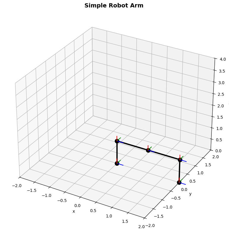
The hierarchy: Our robot arm has the following layout:

root → base → joint1 (+1 in z) → joint2 (+1 in x) → joint3 (+1 in x) → hand (-1 in z)

Create a RobotArm data structure

To manage the robot’s joints and visualize them, we create a RobotArm class that stores all joint frames and provides plotting functionality.

@dataclass
class RobotArm:
    joints: list[Frame]

    def plot_robot(self, axes, color="black", alpha=1.0, show_gismo: bool = True):
        """Plot the robot arm by connecting joint origins."""
        origins = np.array([joint.origin_global for joint in self.joints])
        axes.plot(*origins.T, marker="o", color=color, alpha=alpha, ms=10, lw=3)

        if show_gismo:
            for joint in self.joints:
                plot_gismo(joint, axes, alpha=alpha)
        return axes

    def __getitem__(self, index: int) -> Frame:
        return self.joints[index]

    def __len__(self) -> int:
        return len(self.joints)


def plot_gismo(frame: Frame, axes, scale: float = 0.2, alpha: float = 1.0):
    """Visualize coordinate system axes (x=blue, y=green, z=red) at frame origin."""
    x_axis = np.vstack(
        [frame.origin_global, frame.origin_global + frame.x_axis_global * scale]
    )
    y_axis = np.vstack(
        [frame.origin_global, frame.origin_global + frame.y_axis_global * scale]
    )
    z_axis = np.vstack(
        [frame.origin_global, frame.origin_global + frame.z_axis_global * scale]
    )

    axes.plot(*x_axis.T, c="blue", alpha=alpha)
    axes.plot(*y_axis.T, c="green", alpha=alpha)
    axes.plot(*z_axis.T, c="red", alpha=alpha)
    return axes

The RobotArm class:

• Stores joint frames in a list

• Provides plot_robot() to visualize the arm by connecting joint origins

• Supports indexing (robot[i]) to access individual joints

• Uses joint.origin_global to get the global position of each joint

Build the robot instance

robot = RobotArm(
    joints=[robot_base, first_joint, second_joint, third_joint, robot_hand]
)

Visualize the initial configuration

fig = plt.figure(figsize=(10, 8))
ax3d = fig.add_subplot(projection="3d")

ax3d.set_xlabel("x", fontsize=10)
ax3d.set_ylabel("y", fontsize=10)
ax3d.set_zlabel("z", fontsize=10)
ax3d.set_xlim(-2, 2)
ax3d.set_ylim(-2, 2)
ax3d.set_zlim(0, 4)

robot.plot_robot(ax3d)

ax3d.set_title("Simple Robot Arm", fontsize=14, fontweight="bold")

plt.tight_layout()
plt.show()

Animate the robot arm

Now we’ll create an animation by rotating different joints over time. We’ll:

1. Rotate the base (rotates entire arm)

2. Rotate joint3 alternately up and down

Each configuration is drawn in a different color to show the motion sequence.

steps = 8
angle_per_step = 360 / steps

transforms = []

# move first joint up
transforms.append([(1, {"y": -45, "degrees": True})])

for i in range(1, steps):
    swing_direction = 1 - 2 * (i % 2)  # alternates between +1 and -1
    transforms.append(
        [
            (3, {"y": swing_direction * 45, "degrees": True}),
            (0, {"z": angle_per_step, "degrees": True}),
        ]
    )

Each transform is a list of (joint_index, rotation_params) tuples:

• Index 0 = base, 1 = joint1, 3 = joint3

• First step: rotate joint1 down by 45°

• Subsequent steps: swing joint3 up/down, rotate base around z

Apply transformations and visualize

fig = plt.figure(figsize=(12, 10))
ax3d = fig.add_subplot(projection="3d")

ax3d.set_xlabel("X", fontsize=10)
ax3d.set_ylabel("Y", fontsize=10)
ax3d.set_zlabel("Z", fontsize=10)
ax3d.set_xlim(-2, 2)
ax3d.set_ylim(-2, 2)
ax3d.set_zlim(0, 4)

colors = plt.cm.viridis(np.linspace(0, 1, len(transforms)))
alphas = np.linspace(0.3, 1.0, len(transforms))

for color, alpha, transform_step in zip(colors, alphas, transforms):
    for joint_index, rotation_kwargs in transform_step:
        robot[joint_index].rotate_euler(**rotation_kwargs)

    robot.plot_robot(ax3d, color=color, alpha=alpha)

ax3d.set_title("Animated Robot Arm", fontsize=14, fontweight="bold")
plt.tight_layout()
plt.show()

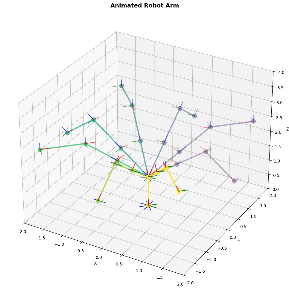
Key observation: The robot arm frames were created once at the beginning. We modify them in the loop with .rotate_euler(), and .origin_global automatically returns the updated positions. No need to recreate the robot or manually track transformations - the frame hierarchy does it for us.

Transforming points through the hierarchy

The real power of frame hierarchies emerges when you need to track objects attached to moving parts. Let’s attach a tool to the robot hand and track its position in world coordinates.

# Tool tip is 0.5 units below the hand in the hand's local coordinate system
tool_tip = robot_hand.point(0, 0, -0.5)

print(f"Tool tip in hand frame: {tool_tip:.2f}")
print(f"Tool tip in world frame: {tool_tip.to_global():.2f}")

# Rotate the third joint - the tool tip position updates automatically
robot[3].rotate_euler(y=90, degrees=True)

print(f"\nAfter rotating joint3 by 90°:")
print(f"Tool tip in hand frame: {tool_tip:.2f}")  # unchanged
print(f"Tool tip in world frame: {tool_tip.to_global():.2f}")  # updated

Tool tip in hand frame: Point(0.00, 0.00, -0.50, frame=hand)
Tool tip in world frame: Point(2.06, -2.06, 2.41, frame=root)

After rotating joint3 by 90°:
Tool tip in hand frame: Point(0.00, 0.00, -0.50, frame=hand)
Tool tip in world frame: Point(1.00, -1.00, 0.91, frame=root)

What happened here:

• We defined tool_tip once in the hand’s local frame

• .to_global() automatically computed its world position through the entire kinematic chain

• After rotating a joint, the same tool_tip object gives updated world coordinates

• The local coordinates remained unchanged (still [0, 0, -0.5] in hand frame)

This is the key insight: define geometry once in the natural reference frame, query it anywhere.

Key Takeaways

Multi-level hierarchies: Robot arms, camera rigs, and mechanical assemblies naturally map to frame hierarchies. Each joint/component is a child of its parent, creating a kinematic chain.

Persistent frames with dynamic updates: Create frames once, modify them later with .rotate_euler(), .translate(), etc. All primitives and child frames automatically reflect the changes through cache invalidation.

Data structures with frames: You can build higher-level abstractions (like RobotArm) that store and manage multiple frames. The frames remain live - calling .origin_global always gives current positions.

Automatic propagation: Define points and vectors in their natural reference frame, then query them in any other frame with .to_global() or .to_frame(). The transformation chain is computed automatically.

Without hazy: Track transformation matrices for each joint, manually compose them in the right order, update dependent transformations when a parent changes, manually transform tool positions through the chain. For a 5-joint arm with a tool, that’s matrix multiplication through 6+ transforms for every query.

With hazy: Define the hierarchy once, modify individual joints freely, query positions anywhere. The library handles composition and propagation automatically.